Volatility Variables, Beta and Risk
It is often said that a picture is worth a thousand words, as shown in the tables and charts below.
Table 1 includes 30 Canadian securities, including five ETFs (lines 17, 18, 19, 20 and 30). In Chart 1 below, the Canadian market is represented by the S&P/TSX60 (XIU ETF).
| Symbol A |
Security Volatility B |
Index (XIU) Volatility C |
Security Beta D |
Specific Risk E |
Systematic Risk F |
|
|---|---|---|---|---|---|---|
| 1 | ABX | 0.46 | 0.07 | –0.56 | 0.91 | 0.09 |
| 2 | AEM | 0.39 | 0.07 | 1.48 | 0.71 | 0.29 |
| 3 | AGU | 0.17 | 0.07 | 0.61 | 0.73 | 0.27 |
| 4 | ARX | 0.25 | 0.07 | 1.74 | 0.48 | 0.52 |
| 5 | ATD.B | 0.25 | 0.07 | – 0.08 | 0.98 | 0.02 |
| 6 | BBD.B | 0.15 | 0.07 | 1.31 | 0.33 | 0.67 |
| 7 | BEI-UN | 0.19 | 0.07 | 0.41 | 0.84 | 0.16 |
| 8 | BMO | 0.10 | 0.07 | 0.89 | 0.36 | 0.64 |
| 9 | BTE | 0.58 | 0.07 | 5.15 | 0.34 | 0.66 |
| 10 | CLS | 0.30 | 0.07 | 0.92 | 0.77 | 0.23 |
| 11 | CM | 0.09 | 0.07 | 1.08 | 0.13 | 0.87 |
| 12 | CNQ | 0.20 | 0.07 | 1.18 | 0.57 | 0.43 |
| 13 | CVE | 0.35 | 0.07 | 1.14 | 0.75 | 0.25 |
| 14 | DOL | 0.14 | 0.07 | 0.08 | 0.96 | 0.04 |
| 15 | ECA | 0.26 | 0.07 | 3.48 | 0.00 | 1.00 |
| 16 | EMA | 0.12 | 0.07 | –0.06 | 0.96 | 0.04 |
| 17 | HGD | 0.72 | 0.07 | 0.38 | 0.96 | 0.04 |
| 18 | HGU | 0.76 | 0.07 | –0.62 | 0.94 | 0.06 |
| 19 | HXD | 0.13 | 0.07 | –1.09 | 0.39 | 0.61 |
| 20 | HXU | 0.13 | 0.07 | 1.13 | 0.36 | 0.64 |
| 21 | MFC | 0.22 | 0.07 | 0.93 | 0.69 | 0.31 |
| 22 | MRU | 0.16 | 0.07 | 0.22 | 0.90 | 0.10 |
| 23 | POT | 0.20 | 0.07 | 0.43 | 0.84 | 0.16 |
| 25 | RY | 0.10 | 0.07 | 0.70 | 0.46 | 0.54 |
| 26 | SAP | 0.20 | 0.07 | 0.79 | 0.71 | 0.29 |
| 27 | SU | 0.18 | 0.07 | 1.10 | 0.54 | 0.46 |
| 28 | TD | 0.08 | 0.07 | 0.82 | 0.23 | 0.77 |
| 29 | TCK.B | 0.49 | 0.07 | 4.16 | 0.37 | 0.63 |
| 30 | XIU | 0.07 | 0.07 | 1.00 | 0.00 | 1.00 |
The tracking error between the index and the XIU is so minimal or nil that we can consider the volatility of the XIU ETF equal to that of the index it replicates.
XIU volatility is, therefore, the volatility reference for the Canadian market. This is important because if the XIU has a volatility of 7% (which has been supposedly consistent throughout the last 12 months) and the return of the ETF in the last 12 months was 7.89% (between the closing price of 12 months ago and the last price, excluding dividends), this represents the benchmark for other securities.
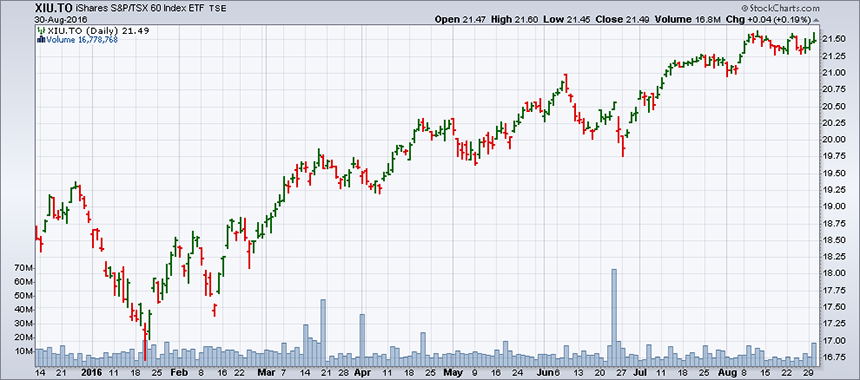
We can assume that if a security has double the volatility, of 14% for example, it should offer double the performance, or 15.78%. At first glance, this deduction is logical, but this is not the case.
We must consider the fact that any company, publicly traded or not, runs two risks: the overall risk (also called "systematic risk"), such as an increase in interest rates, devaluation or revaluation of the county's currency versus others, a postal strike, etc. All companies experience this kind of risk, but each has its own sensitivity to it and its unique way to respond. For example, a company that exports lumber to the United States will be more affected, positively or negatively, by changes in the US/Canada exchange rate than a chain of food stores like Metro (MRU), whose clientele is local.
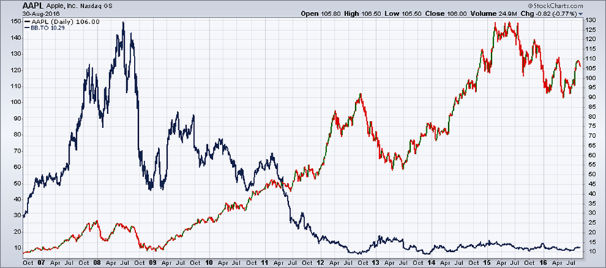
The second type of risk is company specific, which is related to its marketing decisions, its ability to adapt to its customers' changing habits, etc. A typical example of this kind of risk is that of BlackBerry, which did not foresee the threat posed by Apple's iPhone (see Chart 2).
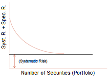
In the 1950s, the father of portfolio management, Harry Markowitz, found that by grouping multiple securities in a portfolio, the specific risk of each security is greatly reduced and can even be brought down to zero. This is shown in Scenario 1: the more securities in a portfolio, the more the downside risk of a security is offset by the positive characteristics of the others.
After building a diversified portfolio which reduces the risk of running a company to zero, all that remains is a security's systematic risk, as measured by Beta (column D in Table 1).
In conclusion, the volatility of a security is divided into two parts: systematic risk and specific risk. The size of one risk relative to the other varies greatly from company to company. This is evidenced clearly by looking at the columns E and F of Table 1. We see, for example, that ATD.B (line 5) has practically no sensitivity to the general market (2%). It is therefore 98% independent. Whatever happens to the market, ATD.B is practically autonomous.
In contrast, the XIU (line 30), consisting of 60 securities represents market risk of 100%; by definition its Beta is 1, and it has no specific risk.
Securities that have a Beta greater than 1 react to market more strongly than the XIU; conversely, those with the Beta is less than 1 are less responsive.
In general, we can say that between two securities with the same volatility (column B), the one with a higher Beta will be more sensitive to fluctuations in the market index. For example, this is the case with ARX (line 4) and ATD.B (line 5).
In general, we can also say that if volatility and Beta (in absolute values) are the same, systematic risk is virtually the same. For example, this is the case with HXD (line 19) and HXU (line 20).
Regarding these two double leverage ETFs in Chart 3; the HXD and its inverse, HXU, it is clear that one is the opposite of the other.
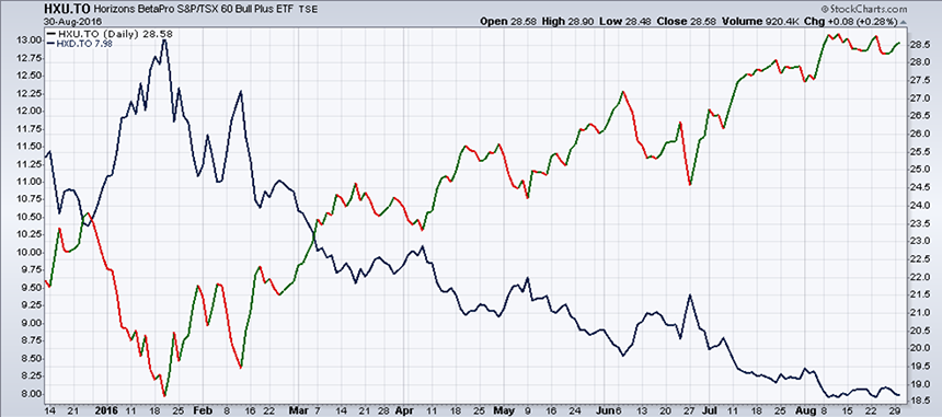
Both ETFs are "constructed" and not a mere imitation of the index. Since the XIU has a Beta of 1, these two ETFs should have a higher Beta and possibly equal to 2 and –2. In fact, the actual Beta of these two ETFs is barely above 1.
This means that investors cannot expect to achieve a "plus" equal to, or almost 2 in the long term. A major reason for this is "risk drag". Table 2 illustrates this phenomenon well.
| Year | Portfolio ABC | Portfolio XYZ | ||
|---|---|---|---|---|
| Annual Return | Value of Portfolio | Annual Return | Value of Portfolio | |
| $100 | $100 | |||
| 1 | 10% | $110 | 30% | $130 |
| 2 | 10% | $121 | –20% | $104 |
| 3 | 10% | $133 | 51% | $157 |
| 4 | 10% | $146 | –12% | $138 |
| 5 | 10% | $161 | 27% | $176 |
| 6 | 10% | $177 | 15% | $202 |
| 7 | 10% | $195 | –7% | $188 |
| 8 | 10% | $214 | 1% | $190 |
| 9 | 10% | $236 | –17% | $157 |
| 10 | 10% | $259 | 32% | $208 |
| Average annual return: 10% | 10% | |||
| Standard deviation (volatility): 0% | 24,4% | |||
| Portfolio value at end of 10 years: $259 | $208 | |||
Table 2 shows two portfolios that are identical at the start. After 10 years, the two have an average yield of 10%. However, the two do not have the same value at the end ($259 versus $208). This difference is due to the fact that the returns from one period to another of portfolio XYZ have been more volatile (24.4%) than those of the portfolio ABC (0%). The depressive effect of volatility shows that the higher the volatility, the lower the yield. "Constructed" ETFs should therefore be considered only for the short term.