The Risk Aversion Coefficient

In the 1950s, when Harry Max Markowitz introduced the concept of "risk" in a portfolio, he inaugurated a sort of modern securities portfolio management. His contribution was crucial to the subsequent development of modern management theories. The fundamental principle that he pioneered is the quantification of portfolio's performance risk.

To measure the risk of financial products relative to performance, we use a measure called the "standard deviation of returns," commonly known as "volatility of returns". In fact, this measure allows us to determine whether a portfolio's performance was consistent over the years or has undergone significant changes. The more risk fluctuated from year to year, the more difficult it is to predict the expected return; a volatile portfolio therefore presents a greater risk than another whose annual return is stable from year to year.

Markowitz went much further by introducing the concept of the "efficient frontier". For example, in a portfolio of two securities whose returns and volatility are known, and in which the price movement of one does not completely influence that of the other, it is possible to calculate the weight of each security in order to achieve maximum performance while taking the minimum risk.

In the chart above, point A (horizontal axis) represents the minimum risk of a portfolio and its corresponding expected return (vertical axis). Applying a mathematical formula shows the percentage of each component in the portfolio. The part of the curve that goes from A to B indicates optimal portfolios with a higher yield, accompanied by gradually higher risk as one moves toward B. The investor can therefore choose the portfolio that suits them best depending on their risk tolerance. All portfolios that range from A to B are optimal. Inside the ABC area, portfolios run a proportionately higher risk without generating optimal performance. For example, at point C there is a high risk with a very low yield.

From an objective and rational perspective, any investor would choose the AB line, which is the ideal portfolio with the minimum risk relative to the chosen level of returns.

The question that arises is, what is the level of risk the investor is able to endure? This is the most difficult question, because the answer is subjective. The ideal portfolio, even that which corresponds to point A, could present a greater risk than an investor is able to bear.

How do we measure the risk aversion of an investor? Several qualitative psychological methods suggest that one should determine what is the most appropriate risk for them, that is to say, decide how much to invest in stocks, bonds and the money market. Some tests help determine the psychological profile of an investor. There are, among others, the PASS test by W.G. Droms, the Baillard, Biehl & Kaiser test - which classifies investors on a scale from "confident" to "anxious" and "careful" to "impetuous"- that of Barnewal which distinguishes between passive and active investors, or the Bonpian test, with eight types of investor. The oldest rule is based on the following equation: 100 – age = the percentage to invest in equities, as the latter are expected to be riskier than bonds.

A quantitative and practical method is the following: we attributed a number from 1 (lowest risk aversion) to 5 (highest risk aversion) to an investor. We then assign this number the letter A, which is called the "risk aversion coefficient".

To get it, we use the following utility formula^{footnote 1}: U = E(r) – 0,5 x A x σ².

In this formula, U represents the utility or score to give this investment in a given portfolio by comparing it to a risk-free investment, such as treasury bills.

E(r) is the expected return of the portfolio and σ2 (sigma squared) is the square of volatility (the square of portfolio risk as defined above).

The part of the equation to the right of the "minus" sign indicates the risk of the strategy itself, taking into account the investor's risk aversion. The formula as a whole therefore gives us the difference between the total expected return of a security (or portfolio) and the risk involved. In fact, by subtracting risk from the expected return E(r), we get the return on a risk-free investment.

The investor can apply the formula using a simple calculator, providing them with a rational approach to choosing a security for their portfolio. The formula requires not only know the security's performance, but also its volatility (or risk) and one's own aversion to risk, on a scale of 1 to 5.

Here are two examples of this formula in use:

Example (i):

• Firsk-free interest rate (Treasury bills): 3%
• Expected return of the portfolio: 6%
• Risk aversion coefficient: 2
• Volatility of security returns: 16%

Applying the formula, we get:

Utility score of investment = 0.06 – 0.5 x 2 x 0.16²= 3.44%

This result means that by subtracting the portfolio risk (adapted to the investor's risk aversion) of the expected result, there is a risk-free return that generates a higher return than Treasury bills (3%). So if risk is equal, investing in this portfolio is better than investing in Treasuries.

Example (ii):

• Firsk-free interest rate (Treasury bills): 3%
• Expected return of the portfolio: 6%
• Risk aversion coefficient: 3
• Volatility of security returns: 16%

Applying the formula, we get:

Utility score of investment = 0.06 – 0.5 x 3 x 0.16²= 2.16%

This result means that by subtracting the portfolio risk (adapted to the investor's risk aversion) of the expected result, there is a risk-free return that generates a lower return than Treasury bills (3%). If risk is equal, it is more profitable to invest in treasury bills than in this portfolio.

The problem of answering the following question remains: on a scale of 1 to 5, which number (A) should we assign to the risk aversion of an investor? On average, we could assign an A of 2.5.

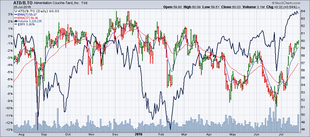
If we apply this formula to an investor with A=2.5 who wants to invest in Couche-Tard Class B shares (see chart below), we would see by applying the formula whether they should put their money into this security. Let's see.

In the past 12 months, this stock has increased by only 3% (left vertical axis). Historical volatility, which is found on the Montreal Exchange website, is 22.58%, and the risk-free interest rate for one year is 0.51%, according to the Bank of Canada.

We apply the formula^{footnote 2:}

Utility score of an investment in Couche-Tard : 0.03 – 0.5 x 2,5 x 0.2258²= – 0.0337 = – 3.37%

At risk parity for the investor where A=2.5, investing in Couche-Tard is much riskier than investing in one-year treasury bills (0.51%).

If risk aversion is minimal (A=1), Couche-Tard is still less attractive than one-year Treasury bills, as shown in the following calculation:

Utility score of an investment in Couche-Tard : 0.03 – 0.5 x 1 x 0.2258²= 0.0045 = 0.45%

Despite the popularity of this stock, we see that its returns over the last 12 months are low. By assuming that the expected returns of this stock for the next year is the same as the last 12 months, even the most risk-tolerant investor should consider avoiding this stock with the current risk and return conditions.