The Free Meal and the Sharpe Ratio
For decades, saloons in Canada as well as the United States offered a free lunch to patrons who had purchased at least one drink. At the time, several religious organizations opposed this practice, judging it as immoral. Using the slogan, "There's no such thing as a free lunch", they explained that in the end, patrons pay for their meal and more by spending money on alcohol.
In the stock market, a fictitious free meal could be compared to a promise of easy income. Does it exist? Probably. For example, a security that offers returns of 9% per year surely represents a high risk: the issuing company is likely embarking on projects that would in practice be unfeasible, at least in the short term. As a result, the value of these shares may fall well below the price the investor had paid.
The 1990 American Nobel Laureate in Economics, William F. Sharpe, is one of the main architects of the modern theory portfolio management. Among other things, he developed a ratio to measure the performance of a portfolio. Sharpe also contributed to the creation of the CAPM (Capital Asset Pricing Model) business model in 1964. This is a standard tool for calculating the theoretical yield required of a security.
All investors should be familiar with the Sharpe ratio: it is simple and useful because it establishes the relationship between the yield and risk of a security. Thus, it allows us to compare performance and risk, a relationship that is not always emphasized in investing. For example, a mutual fund may publish its average annual return over the past five years as 12%, but will not mention the level of risk investors took to achieve this. The logic is that the greater the yield, the greater the risk should be. However, one could actually end up with a very low profitability investment with a high level of risk.
Thinking of the building and management of a portfolio of securities or ETFs, the most known variables are yield and risk. While the performance is intuitively understood, risk is often difficult to grasp. It is called "standard deviation" (or volatility) and represents the variability of returns over time. For example, in the table below, there is a series of 10 annual returns. Portfolio A shows a constant annual return of 10% and with no volatility. Portfolio B has significant variations from one year to another, with a volatility of 24%. Note that the average annual return of the two portfolios is the same. Despite this, Portfolio B generates less money than Portfolio A, as the table shows. In this case, higher volatility has not been accompanied by greater yield.
The Depressive Effect of Volatility
| Year | Portfolio A | Portfolio B | ||
|---|---|---|---|---|
| Annual Return | Portfolio Value | Annual Return | Portfolio Value | |
| Not applicable | Not applicable | 100 | Not applicable | 100 |
| 1 | 10 % | 110 | 30 % | 130 |
| 2 | 10 % | 121 | -20 % | 104 |
| 3 | 10 % | 133 | 51 % | 157 |
| 4 | 10 % | 146 | -12 % | 138 |
| 5 | 10 % | 161 | 27 % | 176 |
| 6 | 10 % | 177 | 15 % | 202 |
| 7 | 10 % | 195 | -7 % | 188 |
| 8 | 10 % | 214 | 1 % | 190 |
| 9 | 10 % | 236 | -17 % | 157 |
| 10 | 10 % | 259 | 32 % | 208 |
| Portfolio A | Portfolio B | |
|---|---|---|
| Average annual return | 10% | 10% |
| Standard deviation (volatility) | 0% | 24% |
| Portfolio value after 10 years | $259 | $208 |
The definition of volatility is somewhat complicated. It tells us that 2/3 of individual yields used in the calculation fall between 10% (the average) ± 24%, i.e. between +34% and -14%. The greater the volatility; the greater the yield oscillations.
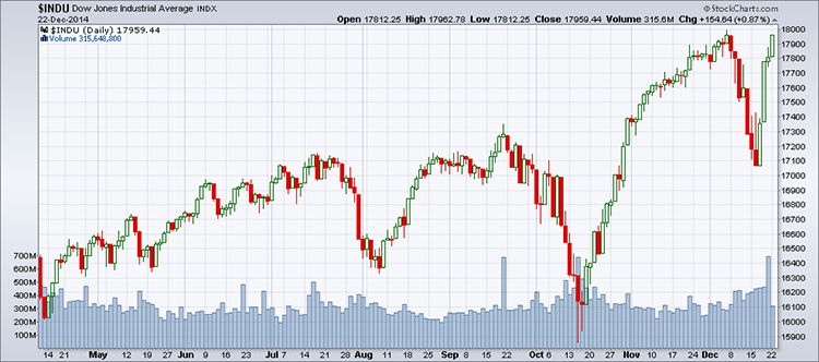
As an example, a rather unusual case of turbulence is one we experienced in December 2014 (see Chart 1). The Dow Jones Industrial Average fell 890 points in seven trading sessions and regained 736 points in the following three sessions, approaching its previous record set on December 5. Between late September and early December 2014, we saw a similar case, but extended over several sessions.
The Sharpe ratio formula as follows: the portfolio return less the return on Treasury bills, the
result of which is divided by the volatility of portfolio returns.
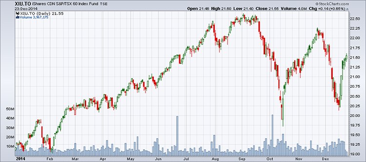
The annualized volatility of the last month is published by the Montreal Exchange for Canadian securities on which there are call and put options. To access this data, investors can visit the Montreal Exchange website. In the "Symbol" field, enter, for example, XIU. The resulting page shows a list of call and put options. At the top of this list is the "30-day historical volatility." At the time of this writing, the volatility of XIU was 15.91%.
For US securities, volatility is published on the www.cboe.com website.
To calculate the Sharpe ratio for the XIU, in addition to volatility we need to know the performance, for example, for one year as well as the yield on Treasury bills.
The formula for calculating return is as follows: the final price less the original price plus
dividends, the result of which is divided by the original price.
To get the XIU's return over the past year (December 2013 to December 2014) we must know:
Price at December 24, 2013: $19.17
Price at December 23, 2014: $21.55
Annual dividends (approximately): $0.50
The XIU's return over the past year was:
(21.55-19.17+0.50)/19.17 = 15.02%
To get the return on Treasury bills, we check the Bank of Canada website. Click on the "Statistics" tab, then "Money Market Yields". On the resulting page, look for "Treasury Bills - 1 Year." At the time of writing, the posted rate was 0.98%.
We now have all the elements to calculate the Sharpe ratio according to the formula above.
(15.02%-0.98%)/15.91% = 0.88
The Sharpe ratio of the Canadian market as symbolized by the XIU and based on historical data is 0.88. This is the reference. To judge whether any other portfolio was better than the Canadian market, the Sharpe ratio of that portfolio must be higher than the market's in order to indicate that the risk-return relationship is advantageous (less risk, higher return).
Take for example the XSP, which is the ETF for the US S&P500 available in Canada, in Canadian dollars. It is very useful because the Canadian investor does not have to worry about exchange rates as this risk is assumed by the issuer of the ETF (BlackRock).
The Montreal Exchange shows that the volatility of this ETF is 13.53%.
The performance data during the same period as the XIU is:
Price at December 27, 2013: $20.93
Price at December 24, 2014: $24.20
Annual dividends (approximately): $0.35
Using the returns formula above, we get:
(24.20-20.93+0.35)/20.93 = 17.30%
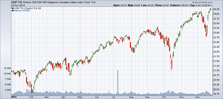
The Sharpe ratio for the XSP is therefore:
(17.30% - 0.99%)/13.53% = 1.21
Conclusion
The Sharpe ratio for the XIU is 0.88, while the Sharpe ratio for the XSP is 1.21. The conclusion is that having invested in the XSP in 2014 involved less risk (lower volatility) with a higher yield than investing in the XIU.
Investors have every interest to include this ratio in their selection criteria for stocks, ETFs or mutual funds in order to gain a more rational view of the relationship between risk and return.
Our examples were taken from data that is easy to obtain for investors, but they are not necessarily those that financial institutions may use (notably volatility, interest rates and dividends). However, the result, that is the comparison between two Sharpe ratios calculated using the same method, is a valid indicator. Naturally, the Sharpe ratio may change with market fluctuations.
Sharpe ratios on ETFs are available on the https://ca.finance.yahoo.com website (enter ETF symbol and from the Summary page, click on "Risk" in the left menu). All mutual funds also have a Sharpe ratio. Just ask for it, and then compare it with the market in general.